Saturday, 7 June 2014

What's Up With The Fake Coin Problem?!


The fake coin problem goes like this: you have a heap of coins but one of them is fake and you know it has a different weight to the real coins. Luckily you have a balance with you, and the aim of the problem is to find out which coin is fake in the least amount of balance-uses as possible.

Let's start with a simplified version of the problem: you know for a fact that the fake coin is heavier. When I first considered the problem I thought-up the following algorithm:

0) start off with a pile of coins in the 'unknown' pile
1) get any two coins and compare their weights
2) if one is heavier, that's the fake coin, and if not, put both coins in the 'real' pile.
3) repeat step 1
4) if there are no coins left in the unknown pile and you haven't found the fake coin, get a better quality balance.

So if you have n coins it's going to take n/2 comparisons in the worst case meaning my algorithm has a time complexity of O(n). Not too bad, but the ability to compare the weights of several coins at once using the balance makes me think there's a better way of cutting down the problem.

It's often a good idea to consider smaller versions of the same problem in order to make an algorithm to handle all possibles sizes. The ideal size to work with is 3 coins: 2 real, 1 fake. You would need to compare two coins and if one's heavier then you know that's the fake coin but if they are both balanced then you know the coin that isn't being balanced (the coin in the unknown pile) must be the fake coin. This can be extrapolated to larger numbers of coins. Lets say I have 9 coins, I can just split that into 3 groups of 3 coins and compare the groups. Just like before, if the two groups I compare are equal in weight then they contain only real coins meaning the fake coin must be in the other group. Because this group has 3 coins we can repeat the process using the same method until we find the fake coin.

Let's try to get this algorithm into some pseudocode. The input is a list of n coins with each value corresponding to their weight. We'll say that our algorithm is only allowed to compare two values or groups of values in the list at a time, which can be done via my 'FindHeavier' function. Our 'FindHeavier' function simply compares the weight of the two sections of the list and returns the heavier one and if they are of equal weight, the function returns -1, but I'll omit it from the code because it's not really important for what we're doing (dat abstraction). Now, considering our 'groups' of coins will be merely sections of the list, we need some notation for specifying a certain range of elements from within out coin list. The way python and C++ does it (and I'm assuming some more languages) is along the lines of L[a..b] where 'a' is the index of the first element of the list L and b-1 is the index of the last element in the range. L[a..b] means "make a new list with the elements with index 'a' through to 'b' including 'a' but not including 'b'". As an example if L = [5,3,7,4,1] then L[0..3] = [5,3,7] i.e. the elements of indexes 0,1 and 2. Why not include both 'a' and 'b'? Let's look at some benefits: If you have a list L of length n you can choose some index 'b' in the middle to split it with and then assign L[0..b] to 'firstHalf' and L[b..n] to 'secondHalf' where the actual element with index 'b' will only show up in secondHalf (meaning there's no overlap), so in that sense it looks pretty clean. Also if you want to know how many elements will show up in your new list, L[a..b], the answer is just b-a. An extra thing to note is that L[i..i+1] will have 1 element so we'll say L[i..i] is an empty list.

We'll be specifying the three group ranges in the code i.e. L[0..a], L[a..b] and L[b..n] and we need to find a way to express a and b in terms of n. We want all three groups to have the same amount of coins in each but if that's not possible (i.e. n % 3 != 0) we can leave the extra coins with the third group so that the two groups being compared have the same number of coins (meaning the weight comparison will actually be helpful in finding the fake coin). Let's look at a list with 9 elements (the contents of each element are unimportant for now):


Starting with 'a', we have n = 9 elements and end up with a=3. This makes me think a=n/3. In turn, b=2n/3. Sounds reasonable, let's look at a list with 10 elements.


This time n = 10 so we can't just say a = n/3 because n/3 = 3.333. But we can floor it to get 3 so let's say a = floor(n/3). Likewise, b = floor(2*n/3). How about a list of only 2 elements. In this case we want the first group to consist of the first element and the second group to consist of the second element, because one of them will definitely be the fake coin so we don't need to worry about a third group. As for the third group, we don't really care how many elements end up in it through our notation because our algorithm will return the solution without needing to ever consider the group.


With our previous definition of a, a = floor(n/3). In this instance a = 1 and n = 2. floor(2/3) = 0. Hmm. What about a = floor((n-1)/3)+1. so when n = 2, a = floor((2-1)/3)+1 = floor(1/3)+1 = 0+1 = 1. This works, but does it work for the above examples? Initially we had n = 9 and a = 3. floor((9-1)/3)+1 = 2+1 = 3. So far so good. What about n = 10 and a = 3? floor((10-1)/3)+1 = 3+1 = 4. Nope. If we just say that a = floor(n/3) and b = floor(2*n/3) then a = b = 0 and as L[0..0] is an empty list, the first two groups are empty and the third group contains the two elements, which is not what we want (because our code is only expects to compare the first two groups). Here's what using the floor(n/3) and floor(2n/3) actually gives us:


But then why do we get this outcome? The reason is that by flooring the n/3 or 2n/3 we ensure that the first two groups have an equal number of elements and the third group has either an equal number of elements or 1 or 2 more due to the extras that get ignored in the flooring process. This means when we have 2 elements the only way to satisfy this condition is to have the first two groups have 0 and the third group to have the 2 leftover elements. SO the way to solve this problem is to go from having the third group getting an equal number of elements + leftovers to having an equal number or less. We can use the ceiling function to help us with this. Let's say a = ceil(n/3) and b = ceil(2*n/3). Now when n = 2, a = 1 and b = 2. When n = 9, a = 3 and b = 3. When n = 10, a = 4 and b = 8.

The reason that switching from floor to ceiling changes the amount that the third group has is that with the floor function you just assume that the list is divisible by 3 and act like there are less elements than there really are meaning the third group gets the equal number of elements plus the 1 or 2 extras. The ceiling function does the opposite by assuming you have more elements than you really do and by the time you get to the third group, it pays the price by having equal-to or less-than the number of elements of the first two groups. Let's go back to our examples and see what the look like now:

Our n = 9 is exactly the same:


Our n = 10 is not:


This may look a bit imbalanced but the difference in size of the first two groups and the third will never exceed 2 elements (because as soon as the difference is three the algorithm will distribute those three elements evenly between the groups).

.... And our n = 2 is looking the way we originally wanted it:


So there we go we have got this list-splicing down-pat. So finally here is the pseudocode.

0  FindFake(L):
1  {
2      heavierGroup <-- FindHeavier(L[0..ceil(n/3)],L[ceil(n/3)..ceil(2*n/3)])
3      if (heavierGroup != -1) return FindFake(heavierGroup)
4      else return FindFake(L[ceil(2*n/3)..n])
5  }

So here we have a neat recursive function which, with each recursive call, cuts the problem down by a factor of 3 (assuming n % 3 = 0 for a particular recursion). This means we have a complexity of O(log3(n)) which as I explained in the complexity post, is just O(logn). Very nice.

This post has really been more of an exploration of splicing lists into equally sized groups than it has been about the fake coin problem itself, but hopefully you've learnt something. I'm thinking next up I'll do a tiny post on invariants and then some bigger posts on trees like heaps and binary search trees and spanning tree algorithms.

Sunday, 1 June 2014

What's Up With Complexity?!

Well I said my next post was going to be on binary and whatnot but I decided to space out the more interesting topics and settle with something dry like data structures. And then I remembered how I cannot be bothered making a post on data structures so I reverted to the idea of doing something fun and settled on complexity.

Complexity is just a solid way of measuring the rate at which an algorithm's processing time will increase with an increase in the size of the input. I'm going to be talking here mostly about inputs which are lists and also some graphs, because these have fairly variable sizes and thus the running time of algorithms which take them as input are very dependent on that size.

We'll start off by talking about running time. This is just the time measured in (hopefully) seconds that an algorithm takes to produce an output given some input. This is going to be dependent on all sorts of things like how fast your computer's processor is, the size of your input (consider the time taken to sort a list of 2 elements compared to 1 million elements), the quality of the code after compilation, and the algorithm's time complexity. Now if we used running time to compare the efficiency of two different algorithms, you'd need to test them on the same machine with the same inputs etc which isn't a very convenient method of comparison (albeit it's certainly more rigorous). The time complexity is the part which is solely dependent on the algorithm, or at least it's dependent enough for you to easily compare between different algorithms.

The time complexity of an algorithm is a measure of the speed of an algorithm as a function of the size of the input, given some abstract machine to work with. What do I mean by abstract machine? Well there may be some processor architectures which are optimised for doing different things like for example the EXAMPLE2000 processor can assign one variable to another in no time whatsoever but takes an entire year to process a simple multiplication, whereas the ANOTHEREXAMPLE3000 processor can do pretty much everything in a millisecond but printing expressions takes a week. The 'abstract machine' is just some model for the time cost of everything that your algorithm can do. Now I know above I said that the time complexity doesn't care about the speed of your processor as they are both components of the 'running time' which is true; e.g. you can have the same processor but one's overclocked. But you still need to use an abstract machine as a framework to determine the relative time cost of everything that your algorithm does.

We're going to use a simple but fairly representative abstract machine where each assignment (x<--y), print, return and comparison (x<y) takes one step (where a step is some unit of time that we can use for comparison). Operations won't have any time cost (this part is not representative but wherever you see operations there'll be an assignment or comparison nearby anyway so we'll consider them covered). Also this will be a random-access machine meaning accessing memory also has no time cost. Also our machine can't do anything fancy like automatically swap elements in a list; it's basically bare-bones in terms of functionality (but don't worry it's not like it's assembly language which I will be doing a post on in the future and it's going to be awesome).

Okay let's have a look at a simple algorithm: the Power(x,n) algorithm which takes x and n and outputs x^n.

Power(x,n):
value <-- 1 //assignment so +1 to time complexity
k <-- 1 // another +1
while (k<=n) do { //comparison so +1
    value <-- value * x //assignment so +1
    k <-- k + 1 // another +1
}
return value //return statement so +1

Alrighty how many steps did we count? 1+1+1+1+1+1 = 6 steps. But hang on, we ignored the fact that there's a while loop in there meaning that part of the code can be executed multiple times. The question is how many times will it be executed? k starts at 1 and gets incremented at the end of the loop so if n is 3 it's going to be incremented 3 times because after the second time k=n so k<=n is true. So the three +1's that form the steps in the loop occur 3 times however there is then another +1 when the while loop checks whether k<=n and finds out that k is larger than n. So now what do we have, 3 +1's outside the loop, 3 as part of the loop which runs three times so that's 3*3 and then an extra +1 on the final comparison of k and n. This leaves us with 3*1 + 3*3 + 1 = 13 steps. But this was for when n=3, so the general expression would be 3*1 + 3*n + 1 = 3n+4. We can call the time complexity t(n) so for this algorithm t(n)=3n+4.

I'm going to make a digression here and say that finding out how many times a loop is going to execute sucks but you don't need to always say something like 'what if n=3?' such as what we did above. There are only a few possibilities of what the conditions of the loop are: you can have k<n or k<=n and you can have k start off being 0 or 1. We can display the number of loops involved in each case using a table:


What about with do-until loops? If we have a loop like this:

k <-- 1
do
    //insert code here
    k+ <-- k + 1
until k = n

then you're going to have n-1 loops (and thus if k<-- 0 at the beginning you'll have n loops). In that sense do-until loops are identical to while loops with a k<n comparison except that with do-until loops there will always be at least 1 loop no matter what because the loop condition occurs at the end of the loop.

Alright one more digression (but this one is a bit more important), if you are counting the steps in an algorithm and come across something like this:

1    if (a<b) { 
2        do something worth 1 step
3    }
4    if (a>b) {
5        do something else worth 1 step
6    }

you might be tempted to count 4 steps here but in fact at most 3 steps can be counted because if a<b then your processor will just skip line 5 meaning that step isn't counted and if a>b then line 2 will be skipped, and if a=b both lines 2 and 5 will be skipped. So here we can say the worst case scenario (a<b or a>b) is 3 steps and the best case scenario (a=b) is 2 steps. If not otherwise specified, any discussion on running time/time complexity refers to the worst case scenario.

Anyway those two digressions illustrate well that the nuances of loops and if statements suck and it would be great if there was a way to not have to worry about them. Well it just turns out that asymptotic analysis is the perfect tool for ignoring those kinds of things. Asymptotic analysis is all about describing the rate at which an algorithm's running time grows for large values of n. Looking at the result of t(n)=3n+4 from above, we can see that for enormous values of n, the 4 doesn't really make much of a difference. That is, the leading n term becomes a better and better approximation of the real value of t(n) as n becomes huge. If we take n=2, t(2) = 6+4 = 12 and simply 3n = 3*2 = 6. So here our approximation differs by a factor of 2. But if we take n=10,000, t(10,000) = 30,000 + 4 = 30,004 whereas simply 3n = 30,000. Here they don't differ by a pathetic factor of 1.0001.

What if an n^2 term showed up in our t(n) function? How could an n^2 term show up? We could have a nested loop, something like:

poweroftwo(n):
value <-- 1
k <-- 1 
while (k<=n) do {
    l <-- 1
    while (l<=n) do{
        value <-- value + n
        l <-- l + 1 //holy crap 1 and l are similar in this font
    }
    k <-- k + 1
}
return value

So outside all of the loops we have 3 +1's and for the outer while loop you've got a comparison and an assignment so that's 2 +1's per loop (and an extra +1 for the last k<=n check) and for the inner while loop you've a comparison and 2 assignments meaning 3 +1's per loop (and an extra +1 for the last l<=n check). So you've got 3 + [n*(2 + [n*(3) + 1]) + 1] where [,] are around each while loop and (,) are around the code in the loop not including the final check. So all in all we'll have t(n) = 4 + n*(3+3n) = 3n^2 + 3n + 4.
Now like above, the 3n and 4 terms don't really matter once n becomes huge because the factor between them becomes smaller and smaller. (the difference gets bigger but not fast enough for the factor to actually increase between them). Consider the graphs of t(n) against n for small values of n:


Compared to large values of n:


So what does this tell us? If we want to be able to efficiently measure algorithmic time complexity, all we need to worry about are the leading terms in our time complexity functions, because these will always dominate as n becomes larger. 

There is a problem with just choosing something like 3n^2 to compare different algorithms which is that in reality different machines will have different ways of implementing algorithms meaning that '3' could be a '2' or a '10' on some other machine. In our case there were three steps in the inner loop but we ignored all the operations like +,* etc so that 3 in 3n^2 could be completely different in reality. If you wanted to get that specific you really would need to look at the architecture of the processor you intend on using. Although the '3' is arbitrary, the n^2 is not and I doubt there's a processor in the world which can turn that n^2 into an 'n' or a constant. But the n^2 is all you need to understand how the running time of the algorithm grows as n becomes large. Luckily for us, when you're comparing two time complexities on different orders, e.g. one has an n^3 leading term and the other has an n^2 leading term, you are guaranteed that past some value of n, regardless of all the constant factors, the time complexity containing the n^3 will become be on top.

A more formal way of saying 'on top' is that our function of a higher power of n will be an 'upper bound' of the function with the lower power. This is where big O notation comes in. We say that t(n) ϵ O(f(n)) if there is some constant C and some value L for which C*f(n) > t(n) for n > L. 

For the t(n) we obtained above: 3n^2 + 3n + 4. We can say this is an element of O(n^2). Because if you said f(n) = n^2 and then gave it a constant factor like 4 then after some value of n it's always going to be above t(n). If we gave it a factor of 3 that 3n+4 would stop our f(n) from being an upperbound, so that extra n^2 in 4n^2 covers those smaller terms as we know n^2 will get larger than 3n+4 as n becomes large. Here's a graph showing this:


You might be thinking 'surely I can just say f(n) = n and make C so big that C*f(n) will always be an upper bound for t(n), which makes this whole big O notation pointless!'. I know that's what I thought when I started learning about big O notation, but the fact is that no matter how large you make your value of C, the function with the higher order will always end up on top, the only thing that's going to change is the value of L.

Let's see if we can say that our t(n)  ϵ O(n) when we say f(n) = n and C = 1000 i.e. we have 3n^2 + 3n + 4 competing against 1000x.


Looks convincing, but let's zoom out:


BAM. Looks like here, L is ~330. What matters is that with a larger leading term, coefficients do not matter for large values of n.

The second thing you might be thinking is the converse of this: can't we just choose our f(n) to be stupendously large meaning we end up with something like t(n) ϵ O(n^n^n^9001). Well yes, we can. It's completely within the definition of our big O notation, but that doesn't make it very useful to say. Big O notation started off in mathematics and has been translated to computer science but I don't think in mathematics they were particularly concerned in whether the C*f(n) was the least upper bound of t(n), all they cared was that after some point n=L, C*f(n) was an upper bound. In practice, we do want to express our time complexity function t(n) as an element of the set of all functions with the same approximate rate of growth for large values of n, but in theory, big O notation is more about expressing our t(n) as an element of the set of all functions which are eventually bounded by C*f(n). So when I say 3n^2 + 3n + 4 is an element of O(n^2) I really mean it just grows in the same way that n^2 does for large values of n, even though I'm theoretically allowed to say it's also an element of O(n^10).

For our algorithm with the nested loop, we would say its complexity is O(n^2) (i.e. its time complexity function can be bounded by n^2 times some factor). For a single loop we would say its complexity is O(n). Let's look all the common complexity 'classes', in order of increasing complexity:

constant                O(1)
logarithmic            O(logn)
linear                    O(n)
superlinear            O(n*log(n)) (also known as linearithmic which is a blend of linear and logarithmic)
quadratic              O(n^2)
polynomial            O(n^c)
exponential           O(2^n)
factorial                O(n!)

O(1) applies to any algorithm whose running time is independent of the input e.g. some algorithm like 'PrintTimeOfDay' which doesn't even take input, or an algorithm which adds two values a and b.

O(logn) shows up in divide-and-conquer algorithms where with each recursion/loop you're breaking down the size of the problem by a constant factor. In a binary search, that factor is 2. Worst case scenario, you don't even find the target, meaning you halved the number of elements in your sublist until you got to one element and then you worked out the element isn't the one you're searching for. Let's say you start off with n=16 elements and you're searching for an element like '1' when the lowest in the sorted list is '2':
We started with n=16 elements and got k=5 loops. If we had started with just the 8 elements there would have been one less loop i.e. k=4. And with 4 elements we'd end up with k=3. The relationship here is that n=2^(k-1). Rearranging this we get k=log2(n)+1. This is a pretty good basis for a time complexity function t(n), because the nuts and bolts of the algorithm will only contribute to smaller terms and some constant factors e.g. maybe each full loop cost 5 steps meaning our t(n) would be 5*log2(n)+1. But clearly the leading term here is log2(n) so we can say that t(n) ϵ O(log2(n)). But above, the complexity class which divide and conquer applies to is just O(log(n)) and doesn't include the base 2. Why is this? Because you can convert between any two logarithms with different bases simply using different constant factors (and constant factors are discarded in big O notation).

To prove this I'll say loga(n)=C*logb(n) where a and b are different bases and C is some constant. We can divide both sides by logb(n) to get:

loga(n)  =   C
logb(n)

and using some log law whose name I've forgotten, we say:

loga(n)  =   logb(a)
logb(n)

so logb(a) = C. Let's go back to the original equation and substitute that in:

loga(n)=C*logb(n) --> loga(n)=logb(a)*logb(n)

and we know that a and b were just arbitrary bases so logb(a) is an arbitrary constant (it doesn't depend on n) so we've proven that the only difference between two logs with different bases is a constant factor. So we don't need to bother including the base when we express the complexity in big O notation because big O notation doesn't care about constant factors.

We've talked about the worst case scenario but not the best case scenario of binary searches. Best case, like many algorithms, is to just get it right on the first time i.e. in the first loop you immediately work out that the middle element in the list matches your target so you can just output the index of it without doing any extra work. This clearly doesn't depend on the input at all so the time complexity is O(1).

You may be thinking 'what about the average case?'. The average case is not always easy to work out, and may involve running the algorithm millions of times for randomised inputs and getting the big O of the average time complexity. The worst-case complexity is usually a good enough measure of what kind of running times we should expect from an algorithm.

So now we've talked about constant time complexity, logarithmic, we've done linear already, next up is superlinear. This is just a combination of linear and logarithmic, e.g. for every element in the list you need to perform something which has a complexity of O(logn). So far we haven't come across one of these but Binary Trees and Quicksorts both involve that O(nlogn) complexity so I'll go into depth when we come to those.

Polynomial time i.e. O(n^c) where c is some greater-than-1 constant shows up whenever you've got nested loops (just like with quadratic time). However there are some situations like particularly efficient matrix multiplication algorithms which can have complexities like O(n^log2(7)) in the case of 'Strassen's Algorithm'. Here's a good time to mention that due to big O notation being all about upper bound, and with O(anything) just being a set of functions, each big O set of lower complexity is a subset of the sets with higher complexity. For example the running time of logarithmic-time algorithms can be bounded by a polynomial function like n^5 and thus although not polynomial in the traditional sense, logarithmic-time algorithms are considered to be 'polynomial-time' algorithms simply because O(logn) ϵ O(n^c). Any algorithm with a polynomial time complexity is considered pretty good and if you have an algorithm which operates on polynomial time, even if it's n^3 or n^5, it's probably going to perform better than an algorithm which has an n! or 2^n term in the t(n) function, for large values of n.

As for O(2^n), the 2 in that is also arbitrary and all that matters is that it's greater than 1. Why? Because 2^n and 3^n differ by a constant factor (which is being multiplied with n) of log2(3). That is, 2^(log2(3)*n) = 3^n. But this isn't the same kind of constant factor we've seen before because it actually does make a difference to the rate of growth of the running time, due to being part of the exponent. However, as previously mentioned, the coefficients on our n-terms are subject to change depending on the processor, so we consider both the above examples to be equal.

As for situations where O(2^n) shows up, I'll be making a post about the travelling salesman problem which can be solved via 'dynamic programming'. The same problem can be solved using brute force (i.e. generate all the permutations of paths that our salesman can take and then output the valid ones) and if the word 'permutation' gives any indication, the complexity of that particular approach is O(n!). The problems whose best algorithms require exponential, factorial or even greater complexity (something like maybe O(n^n!)) are called 'intractable' problems. 'Intractable' means 'hard to deal with' i.e. for large values of n the running time really gets out of hand fast.

I wanted to show a comparison table of running times for various complexities and values of n but this blog's budget is already cutting enough corners (i.e. I spent 5 minutes looking for it on the internet and couldn't find it) but take my word that for large values of n, exponential and factorial running times are absolutely enormous. I don't care how super your super-computer is, if you can compute one billion steps per second, dealing with an algorithm where t(n) = n! where n = 100, you will still need to wait 100!/1,000,000,000/60/60/24/365/1,000,000,000 = 3*10^132 billion years before your algorithm is done. 

For everything I've said here about time complexity, the same can be said about space complexity. Space complexity is just an expression of the amount of memory you need to be able to use your algorithm e.g. sorting a list of n elements may require O(n) space to be able to store the list in memory whilst it's being used. Luckily with the level of compression technology and data-storage technology we have today, space complexity doesn't need to be considered as often as time complexity, but it still is a factor to consider if you have enormous inputs or enormous temporary chunks of data being used in the algorithm, and if you don't have much space to actually store it all.

Another thing to mention is that n is not always the only thing which can affect the complexity. For graphs where vertices and edges are stored separately, you can have algorithms that have time complexities along the lines of O(E+V). However even for graphs you can just consider n to be E+V, and simplify the problem if you want to.

Now when would using big O notation not prove very useful? As stated above, the notation is best used when looking at large values of n, meaning that some 'higher-complexity' algorithms may in fact have lower running times for very small values of n. Consider n^3 vs 2^n for small values of n. Before 2^n starts really taking off, it's actually underneath its polynomial counterpart and so for those values of n, it would be the better time complexity. This is why people often include multiple algorithms in their code and just switch gears between the algorithms when the value of n reaches the L in the formal definition of big O notation (or at least I think they do because that would make sense).

Also, constant factors often matter a lot, and although I showed you about half-way through this post that 1000x will eventually get overtaken by a higher-order complexity, that doesn't mean that while it's on top, it's  not on top by a very large margin. Again, gear changers would be good here. This applies to the smaller terms in our t(n) function too, as they can dominate the function for smaller values of n, depending on their constant factors.

Algorithms which go to great lengths to lower their complexity often become exceedingly 'complex' in terms of readability and comprehendability (that's not a word? It is now) and if you're working with a team that would rather keep things simple because efficiency isn't that much of a priority, it could be beneficial to just stick to the 'simpler' but more time-complex algorithms. This is a bit of a hilarious contradiction; having the easier-to-understand algorithms being more complex than the harder-to-understand ones, but it makes sense when you consider the usual process of making algorithms is to start off with something intuitive and in the search for more efficient algorithms to solve the same problem, venture further from what comes easily to your understanding.

SO that concludes my enormous post about complexity. I was going to touch on Big Ω ('big omega') and Big Θ ('big theta') notation but I'll save that for another time. Actually they won't take long to explain: basically Big Ω is about finding a lower-bound to an algorithm (the only difference is '>' sign from big O gets flipped) the and Big Θ is the set which is the intersection of the Big O and Big Ω sets i.e. if t(n) is an element of Θ(n^2) then t(n) can be upper-bounded by C1*n^2 where C1 is some positive constant and lower-bounded by C2*n^2 where C2 is some other positive constant. if your function is in Θ(n^2) then you're guaranteed that the highest-order term in your function is some constant times n^2, which begs the question of why we don't use big Θ for everything? Basically the answer is that with big O notation you can categorise complexities into all the higher ones so I can say 'polynomial' includes O(logn) for convenience (well maybe this is more of a weakness than a strength), but more importantly the intersection of all the big O's and the big Ω's isn't that big because you're not always going to have a function which, depending on the constant, can be both an upper bound and a lower bound for your t(n), so we just go with big O notation because in practice it's basically used as if it were big Θ but also for the sake of convenience via just sticking to one kind of notation.

OKAY now I'm done, there you go. Complexity is quite a beast but at the end of the day it's just one of the approaches we have to comparing different algorithms.

Friday, 30 May 2014

What's Up With Combinations With Repetition?!

In an earlier post I talked about combinations and permutations and at the beginning I used the concept of permutations with repetition as a foundation for understanding permutations and combinations without repetition. Today we're going to talk about the missing link: combinations with repetition.

Let's use an example: A guy has 7 dollars and he wants to spend all of it and he goes to a vending machine where each drink (due to some savvy and possibly illegal price fixing) costs 1 dollar each. The guy can choose from water, coke, pepsi and OJ and yes that's canned OJ which will one day hopefully become a reality. So he's got four categories to choose from and seven 'slots' effectively. The problem here is that unlike previous combinatorics problems where you could only use each element once, we can say here that there is an infinite supply of each category (or there are at least seven of each drink in the vending machine; price fixing or no price fixing there is no economical mechanism to create an infinite vending machine). So how can we go about looking at this problem in a way so that there are no repetitions and hence we can use our handy C(n,r) formula?

We can start by just using a tally of how many of each drink the guy can buy:

Water       Coke       Pepsi       OJ
    1             11          111          1      = 7
                 1111         11           1      = 7
   111           1             1           11     = 7

Listing all of these states might take some time, but even if we listed all of them, it's not clear how we can use this layout to end up with something along the lines of C(n,r). How about we represent each of these different states as a bit string, using 0's to represent the transition from one category to another:

Water        Coke        Pepsi         OJ
    1      0      11    0     111   0      1      or 1011011101
            0    1111  0      11    0      1      or 0111101101
   111   0       1     0       1     0     11     or 1110101011

each of these bitstrings will end up with 10 digits; that's 7 for the seven slots we have plus an extra three for each transition (and the #transitions = #categories-1). So if our problem involves 's' slots and 'c' categories, the number of digits we'll have will always be s+c-1.

Should we stop here and say 'well clearly there are 2^10 = 1024 numbers represented by 10 bits so that's the number of combinations we have'? Although the bitstrings are good representations of the problem and every state has a unique representation, you're never going to see a bitstring like 1000000111 because we can only have 3 0's and thus we can only have 7 1's, so we know the number we'll end up with will be less than 1024.

So what can we do? How about we give each place in the bitstring an alphabetical index:

a  b  c  d  e  f  g  h  i  j
1  0  1  1  1  0  1  1  0  1
0  1  1  1  1  0  1  1  0  1
1  1  1  0  1  0  1  0  1  1

Now we can use another way of representing the different states: just find out the positions that the 0's are in. If you came up to me and told me there were ten digits, indexed with letters, and the zeros were in the places {b,f,i} like in the first state, I'd be able to work out that there must be 1 water purchased, 3 cokes, 2 pepsi's and 1 can of delicious OJ. So clearly just using a set of the three positions that the zeros belong to is enough to describe one state:

a  b  c  d  e  f  g  h  i  j
1  0  1  1  1  0  1  1  0  1 --> {b,f,i}
0  1  1  1  1  0  1  1  0  1 --> {a,f,i}
1  1  1  0  1  0  1  0  1  1 --> {d,f,h}

Now we just need to ask how many ways there are of making a set of 3 elements using our 10 letters? Well that's something we can apply the C(n,r) formula to: we have 10 letters and we need to choose 3? That's just C(10,3) = 120. So our guy can walk away with one of 120 possible combinations of drinks. So where do the 10 and 3 come from? As I said above, the 10 is the number of digits in the bitstring which will be the original number of slots (7) plus the number of transitions (#categories-1 = 4-1 = 3). The 3 in C(10,3) is just the number of transitions.

So given a problem where you need to fill s slots with c categories, you can use C(s+c-1,c-1). You may be thinking 'what about that symmetrical property where C(n,r) = C(n,n-r). Well in this case n = s+c-1 and r = c-1 so that translates to C(s+c-1,(s+c-1)-(c-1)) which is 
C(s+c-1,s). What does this mean? Well it means if you tried to find all the ways of putting those 10 letters into a set with 7 slots (one slot for each '1' in the bitstring) you'd get the same number of combinations. Just like above, we can construct a set using all the letters which don't have a corresponding '0' (i.e. they've got a '1'):

a  b  c  d  e  f  g  h  i  j
1  0  1  1  1  0  1  1  0  1 --> {a,c,d,e,g,h,j}
0  1  1  1  1  0  1  1  0  1 --> {b,c,d,e,g,h,j}
1  1  1  0  1  0  1  0  1  1 --> {a,b,c,e,g,i,j}

So each of these sets will also tell me how many of each drink the guy chose e.g. looking at the first set, the 'a' says he got 1 water, then there's a jump to c meaning now he's getting cokes so he gets 3 cokes then there's a jump to g meaning now he's getting pepsi's so he gets 2 pepsi's and then he jumps to j so he gets 1 OJ. Both the sets using the 0s and the sets using the 1s express the exact same information and thus the number of combinations sets using 1s equals the number of sets using 0s i.e. C(10,3) = C(10,7).

So every time you get a question like this you can use C(s+c-1,c-1) or C(s+c-1,s) (or if you're a lazy bastard use your programmable calculator to define something like Cr(c,s)). Pick whichever one feels more intuitive to you (the former is more intuitive for me). You don't need to worry about the difference in computational difficulty because

      10!         =     10!  
  (10-3)!*3!           7!*3!

is exactly the same as

      10!        =      10!  
  (10-7)!*7!           3!*7!

which is the whole reason why the symmetrical rule of combinations exists in the first place!

Another way in which these kinds of problems pop up is where you're told that x,y and z are non-negative integers and you want to know the number of solutions to the equation x+y+z = 12. The vending machine problem could have been expressed like this i.e. if water = w and coke = k (I don't want to make things confusing by calling coke 'c') and pepsi = p and OJ = o then you could say w+k+p+o = 7. So here the number of terms is our 'c' and the number on the right is our 's' so for x+y+z = 12 the number of solutions will be C(12+3-1,3-1) = 91. 

What happens if the numbers can be negative? Well then there'd be an infinite number of solutions e.g. the equation x+y=1 has an infinite number of solutions because you can just keep subtracting 1 from and adding 1 to y and the equation will still hold true.

Alright well what if the equation came with some constraints like x+y+z = 12 and x and y are ≥0 by z is ≥-5? We can just bring the problem back to all numbers being non-negative by simply adding 5 to both sides of the equation by first saying v = z+5 so v ≥ 0 and secondly adding 5 to 12 = 17 so we end up with x+y+v = 17 and we can solve the problem normally just by going C(17+3-1,3-1) = C(19,2) = 171 solutions.

This works for both positive or negative numbers: if you were told in the above problem that y≥2 you could just say m=y-2 and turn the 12 on the right hand side into a 10 so that each variable had the condition of being ≥0. You don't need to go and write out the substitutions, you can just crunch the numbers in your head i.e. x≥4, y≥-3, z≥7 and x+y+z = 10 then 10-4+3-7 = 2 so the answer is C(2+3-1,3-1) = C(4,2) = 6.


We can apply the above logic to a similar vending machine problem where our guy is told he needs to get at least 1 of each drink. This is the same as an equation w+k+p+o = 7 where w,k,p,o ≥ 1. Easy fix, just subtract out the 1's from the 7 leaving you with 7-4 = 3 which leads you to C(3+4-1,4-1) = C(6,3) = 20. The intuition behind this is just that if you know he's going to walk away with 1 coke, pepsi, water and OJ then the only room for combinations is in the three remaining slots so the 4 drinks you know he's going to get don't matter at all hence you consider the number of slots to be 7-4 = 3.

Next up may as well do some more stuff involving bitstrings so we'll look in depth at binary numbers.

Saturday, 17 May 2014

What's Up With Sequential And Binary Searches?!

Searching is something everybody is familiar with; looking up a song in iTunes (Again, I am aware that iTunes is the worst thing on the planet like if I go to use the scrollbar on the right-hand-side of the screen but my cursor is against the edge of the screen it doesn't scroll, I feel like I'm taking crazy pills here) or entering something into a google search are common day activities. In this post I'm not going to attempt to replicate Google's search algorithm but I'll try Bing's. Not really I'm actually going to talk about sequential and binary searches.

Sequential Searches (or Linear Searches) are the simplest form of searching you could think of: start from one side of a list and go to the other side, checking each element to see if your target shows up. It's not very efficient, for example if I have a list of one million items and I'm looking for the element 19102348 (perhaps this is a phone number list) and it happens to be one the opposite side of the list to where I start searching, I'm in for a good time. The only real benefit to sequential searches other than their simplicity is their ability to take a list of any form and find the desired element without messing around with anything.

Binary Searches are more efficient than sequential searches but do indeed do some messing around (note the tactical insertion of the word 'indeed' to avoid saying do do). A binary search only works on sorted lists because its method is dependent on telling whether the target is higher or lower in the list than the element that the search is inspecting. The idea is to begin by selecting the middle element in the list so if the length of the list is n, the item's index will be (n-1)/2 and it'll need to be floored to ensure you don't go looking for an index of 8.5 or something (i.e. to ensure nothing goes wrong if your list has an odd number of elements). So you look at this middle element and determine whether it's larger or smaller than your target. If it's larger, clearly you don't need to bother looking to the right of the element (assuming the list is in ascending order) so you can just focus on the left hand side.

So you now want to treat this new left-hand section of the list as a list in and of itself. You can store a value called 'high' or something which is the highest index in the list (previously it would have been n-1). And now we want it to be one less than the index you just checked (because that index and all those to the right of it were larger than the target). If we're going to have an upper bound variable it makes sense to have a lower bound one too (call it 'low') incase for example the target was larger than the first element we checked and the new list had the same upper bound but the lower bound needed to be changed to 1 greater than the element we checked.

Alright so now the lower bound will be 0 (nothing's changed here) and the upper bound will be ⌊(n-1)/2⌋-1. Now we just repeat the process we did at the beginning; compare the middle element of this section of the list to the target. So the middle (we can call the variable 'mid') will be ⌊(high+low)/2⌋. If the element is the target, we can return its index. If it's larger than the target, we need to look to the left meaning we need to set the upper bound to the middle element's index minus 1 and if it's smaller than the target we need to bring the lower bound to the middle element's index plus 1.

We can repeat the process until the target is found, in which case we return the index of that element. We also need to account for the possibility that the target isn't in the list. Eventually we'll get low = high at some point i.e. there's only one element in our sublist and after the algorithm checks that, if the element isn't the target and it's smaller than the target, low will end up being low+1 and if it's greater than the target, high will end up being high-1. In either case, high will end up lower than low (where in all other circumstances high > low) and it's at that point we can say the algorithm failed to find the target and return -1 (which is the all-encompassing 'I have failed you' return value).

I'll be making a big recursion post later on but for now, we can just say that a recursive function is one which calls itself with slightly modified input.

Let's say our algorithm is called BinarySearch and it takes the arguments 'list' (our list will be called L), 'target' (i.e. the target value), 'low', and 'high'. Our list L will have n elements and thus we can initialise low = 0 and high = n-1. Here's the pseudocode for the algorithm:

Clearly this algorithm will be repeating the same process again and again but on smaller sections of the list (with the range of each section defined by low to high) which begs the question of what kind of algorithm to use. When you find that through your algorithm you create smaller problems similar to the original problem that needed to be solved, recursion is a useful tool to use.
BinarySearch(L, target, low, high) { 

    if (high < low) 
        return -1

    mid = ⌊(low + high) / 2⌋

    if (target < L[mid])
        return BinarySearch(L, target, low, mid-1) //consider left half 
    else if (target > L[mid]) 
        return BinarySearch(L, target, mid+1, high) //consider right half 
    else //the only other possibility is for target = L[mid] in which case y              //you've found your target and can return the index of it i.e. mid.
        return mid 
 }

Let's see what happens with a list like L=[1,4,6,8,9,10,12,15,19,24,30] (it's got 11 elements) when searching for 9. We call the algorithm:

BinarySearch(L, 9, 0, length(L)-1)

First it checks whether high < low i.e. whether 10<0 which it's not so we move on to the initialisation of mid. mid will be ⌊(10+0)/2⌋ = 5 so we're looking at the element with index 5, which is the 10 in the list. Now we see whether the target is less than 10 and it is because we're searching for 9 so we call the algorithm again but now it's:

BinarySearch(L, 9, low, mid-1) where mid-1 is 4 and low is still 0.

We do the high < low check again and it's false again because there's still a chance we can find our target, then we get the new mid which will be ⌊(4+0)/2⌋ which is 2 (referring to the 6 in the list) and now we check whether it's larger than the target and it's not and then we check whether it's smaller than the target and it is so we now only care about the elements between the elements 6 and 10 exclusive. So we call the algorithm again:

BinarySearch(L, 9, mid+1, high) where mid+1 is 3 (referring to the 8 in the list) and high is unchanged since the last call i.e. 4 (referring to the 9 in the list).

We go through again and find out the mid is ⌊(4+3)/2⌋ = 3. The target is higher than this so look to the right by bringing low up to mid+1 which is 4. Again we call the algorithm:

BinarySearch(L, 9, mid+1, high) where mid+1 is 4 and high is also 4 so we've got 1 element left.

The one element we have left is 9 (index = 4) which is luckily the target so the algorithm sets the new mid to ⌊(4+4)/2⌋ = 4 and after working out that the target is neither smaller nor larger than the 9 in the list, it can say 'aha! found it' and then return the index of 4 i.e. 'the element you're looking for has the index of 4 in the list'.

However we're not done because this BinarySearch algorithm is going to return that result to the algorithm which called it and then that algorithm, having now a value to return to the algorithm that called it, can do so and the chain continues all the way back to the very first algorithm we called which then directly returns the index to us. When you have a recursive algorithm whose last action is returning the result of another instance of the same algorithm (which is what we're dealing with here) we call that algorithm 'tail recursive' because the recursion occurs at the 'tail' (i.e. at the end) of the algorithm. This doesn't mean the end as in the last line of code in the algorithm but the last action it performs (for example either of the two BinarySeach calls in the BinarySearch algorithm can be at the tail of the algorithm depending on whichever is called).

Now recursive algorithms are useful in being fairly intuitive to use and often simplistic but in every single case of using a recursive algorithm, an iterative algorithm could be used instead. This is because the recursive algorithms are handled by the CPU as iterative anyway with the assistance of a call stack (I'll write about that later).

The iterative approach to the BinarySearch algorithm is as follows:


BinarySearch(L, target) {

    low = 0 
    high = length(L) - 1

    while ⌊(low <= high)⌋ {        mid = (low + high) / 2 
        if (target < L[mid]) 
            high = mid - 1
        else if (target > L[mid])
            low = mid + 1 
        else 
            return mid 
    }
    return -1
}

luckily for us, this is an instance where an iterative algorithm is a whole lot simpler than wrapping one's head around the recursive alternative. Having said that, the binary search was a good place to warm up for all the recursive algorithms to come

Wednesday, 14 May 2014

What's Up With Combinations And Permutations?!

Combinations and Permutations come up a lot in computer science because we're often dealing with a system that can be in a finite number of states based on the combined individual states of individual elements. For example You may want to know how many subsets of the set {A,B,C,D,E} there are and you could approach this by saying that each element is either in the subset or not (i.e. the state of each element is in/not-in the subset). So you can now go through and work out the possible subsets by considering every permutation of states: (1 = in the subset, 0 = in the subset, NOT)

It's self explanatory here the order is important in permutations because 00001 (E) is different to 00010 (D). The full number of permutations aren't there (because who can be bothered filling all those grid spaces I mean just look how badly aligned they are) but this is a good motivation to calculate the number of permutations without writing them all out.

I'll start by saying that with one bit there are two possible states (0 or 1). With two bits there are 4 possible states (00, 01, 10, 11) and with three bits there are 8 possible states (000, 001, 010, 011, 100, 101, 110, 111). clearly when you append an element which can have k states (in this case 0 or 1), the total possible number of states gets multiplied by k. k in this case is 2 so you start off with 1 element: 2 states, then 2 elements: 2x2 = 4 states, then 3 elements: 2x2x2 = 8 states. The pattern when every element has the same number of states is that the system will have k^n states (which here is 2^n, n being the number of elements).

You've seen this occur with conventional 3-digit padlocks where each digit has the numbers 0-9 (10 possible states) and there are three digits so the total number of permutations is 10^3 = 1000.

In the case with finding subsets of {A,B,C,D,E} there are 5 elements each with 2 possible states hence there is a total of 2^5 = 32 possible subsets.

However permutations often occur in non-repeating form (in fact when you say permutation it's implied you mean the non-repeating form) e.g. you have 3 chairs and 3 people (A,B and C) and you want to know how many permutations there are for sitting positions. The idea here is that in the first chair you can sit A, B or C so there's 3 states already. But for each of those three states there'll only be 2 possible states for the second chair as there are only 2 people left to sit in it. By the time you have 2 people sitting, the third chair only has 1 person left to sit in it and so there is only one state for that chair. What you end up with is 3 x 2 x 1 or 3! states. I'm not being over-the-top here, the '!' means factorial in maths so n! = n * (n-1) * (n-2) ... * 1.

So now we know if there are n people and we need them to sit into n chairs there are n permutations. Again, we care about order and consider A,B,C to be different to A,C,B. If we didn't care about order we'd say there's only one possible state but I'll get to that later.

It's convenient when there's an equal number of people and chairs but what happens when the numbers are different? Lets say there are 5 people and 3 chairs. In the first chair you can sit 5 people so there's 5 states right there, and then you'll have 4 left for the second and then 3 left for the third chair, and the other two don't contribute anything to states because we don't care about the order of the people not sitting in chairs. So now we have 5 x 4 x 3 which is a kind of truncated factorial of 5, but it only has 3 terms being multiplied. What we can deduce from this is that if you have n people going into r chairs just get the first r terms of n! and you'll have your answer. However we want to express this mathematically, so let's give that a try:
5 x 4 x 3 is the same as:

5 x 4 x 3 x 2 x 1
                 2 x 1

because the 2 x 1's cancel out. This is the same as 5!/2! but where did the 2! come from? 2! is the number of chairs you don't have in terms of the total number of people or the number of people minus the number of chairs i.e. 5-3 or generally n-r so the 2! is really (5-3)! or (n-r)!. Which means we can express the number of permutations of n people sitting in r chairs as:

   n!  
(n-r)!

I know that by the time you look at the formula you lose the initial intuition behind just taking the first r terms of n! but remember that's all the formula is.

The situation could also be reversed i.e. you've got n chairs and r people to assign the chairs to (where you've got more chairs than people, say 5 chairs 3 people) and instead of thinking in terms of chairs we think in terms of people: the first person has five possible chairs they can be sitting in so 5 states, then the second person will have 4 possible chairs left to choose and then the third person will have 3 possible chairs left which is 5 x 4 x 3 = 60 which boils down to the same formula above.

Permutations are good when you care about the order of your elements, for example you'll consider ABC to be different to ACB. But what happens when you don't mind what order the elements are in and just want to know how many non-ordered subsets of r elements you can make from a set of n elements. Now we're thinking about combinations. Back to the original chair example you have 5 people and 3 chairs but you don't want there being any double-ups (or triple-ups etc). We know that there are 60 permutations, but how many of those permutations are the same combination?

ABC
ACB
BAC
BCA
CBA
and CAB

are all different permutations but they are the same combination because combinations only care what elements are in the subset, not their order. There are 6 combinations there which all fall under the 1 combination, so wouldn't it make sense to just divide the total number of permutations by 6 to get the total number of combinations? Obviously using ABC is arbitrary and 6 permutations of ABD or ABE will also show up, so it is reasonable to just say there are 60 permutations but for every 6 permutations there is 1 combination so there are 60/6 = 10 combinations:

ABC   ACE   BCD   CDE
ABE   ACD   BCE
ABD   ADE   BDE

But what does this 6 that we're dividing by represent? It is the number of arrangements of any three elements. And when we're talking about arrangements we're talking about order being important which means here, we're just asking how many permutations of three elements are there so I can cancel all the replicates out by dividing the total number of permutations (60) by that number (6). 3 elements with 3 positions, that's going to be 3!/(3-3)! = 3!/0! = 3!/1 = 3! = 3 x 2 x 1 = 6 permutations.

The obvious question is 'why is 0! equal to 1?' and I'll answer it with a bit of maths wizardry. We know 5 x 4 x 3 x 2 x 1 is 5! but it can also be expressed as 5 x 4!. In general n! can be expressed as n x (n-1)!. So 1! which equals 1 can be expressed as 1 x (1-1)! = 1 x 0!. dividing both sides by 1 we get 0! = 1. It's also evident that if you want the permutations of 3 elements in 3 positions, we already know the answer is 6 just by looking at all the permutations so if 3!/0! wasn't equal to 6 (i.e. 0! wasn't equal to 1) that wouldn't make sense.

So to get the final formula for a combination: if you have n elements going into r slots you get the number of permutations i.e. n!/(n-r)! and divide that by the number of permutations of r elements in the r slots i.e.
r!/(r-r)! = r!/0! = r!. So the formula becomes:

    n!    
r!(n-r)!

And thus the only difference between this and the formula for permutations is the r! factor which is used to cancel out the repeating combinations in the set of permutations.

Now we can say that P(n,r) = n!/(n-r)! and C(n,r) = n!/(r!(n-r)!). Also with combinations you can say 'n choose r' to mean C(n,r) as in, you have n elements and you need to find all the ways of choosing r of them i.e. the number of ways you can put n elements into r slots without caring about order.

The second-last thing we need to look at is the symmetry of combinations. For example having 3 elements and putting them into no slots i.e. C(3,0) has 1 combination and the same is true with 3 elements and 3 slots i.e. C(3,3). If there is 1 slot, there will clearly be 3 combinations (A,B, and C) i.e. C(3,1) = 1. And if there are 2 slots, there will also only be 3 combinations i.e. C(3,2) = 1 because in each combination you're really just choosing which element isn't in one of the slots: (BC, AC, BA). What about with 5 elements and 3 slots? C(5,3) = 10 but instead of choosing 3 elements to be in the 3 slots in each combination, you could have just chosen 2 elements not to be in the 3 slots (i.e. the combinations of 5 elements in 2 slots) i.e. C(5,2). Using the 10 combinations of C(5,3) from above, we can compare them to the combinations of C(5,2) in brackets:

ABC(DE)   ACE(BD)   BCD(AE)   CDE(AB)
ABE(CD)   ACD(BE)   BCE(AD)
ABD(EC)   ADE(BC)   BDE(AC)

So asking somebody how many ways there are to have 5 elements and choose 3 is the same as asking them to have 5 elements and choose 2. Or more generally, if you have n elements, choosing r is the same as choosing n-r. so C(n,r) = C(n,n-r). Mathematically speaking, the reason for this is that if you substitute n-r for r in the equation n!/(r!(n-r)!) all that happens is the r! becomes (n-r)! and the (n-r)! becomes (n-(n-r))! which is just r! meaning all you've done is swapped the two terms in the denominator and nothing has changed! This clearly isn't the case with permutations because they don't have an r! in the denominator, meaning something like P(5,3) = 60 but P(5,2) = 20 thus they're permutations aren't symmetrical.

Final thing:

You may have heard of Pascal's Triangle which is a neat way of finding combinations. Until very recently I thought this was a magical triangle which through coincidence (i.e. extremely complicated mathematics) happened to display interesting characteristics of combinations. Namely, that

C(n,r) = C(n-1,r-1) + C(n-1,r)

What does this mean?

Lets say you have n elements and you want to focus on one in particular (we'll call it k). If you have r slots to put the n elements into then obviously there are C(n,r) combinations. But you could also say 'let's consider what happens when k is in one of the slots and when it isn't'. When you ensure k is in one of the slots, the number of combinations that you can get with the remaining elements is C(n-1,r-1) because what you've done is the equivalent of removing an element from the n elements (so now you've got n-1 elements) and you've removed a slot (so now you have r-1 slots). What if you ensured k wasn't in one of the slots? Then you now again have n-1 elements to worry about but this time there are r slots to put those n-1 elements in. Because k can either be in a slot or not in a slot, if you add up these two sets of combinations i.e. C(n-1,r-1) + C(n-1,r) you'll get the same number as if you had just worked it out normally saying there were n elements with r slots i.e. C(n,r). So this is how we know C(n,r) = C(n-1,r-1).

As an example let's do C(5,3). We'll use the set {A,B,C,D,K} (there's a K there instead of an E because we've defined the element to focus on as being k). Working this out normally:

ABC   ACK   BCD   CDK
ABK   ACD   BCK
ABD   ADK   BDK

Ten combinations. Now let's see what we get when we ensure K is in one of the slots?

ABC   ACK   BCD   CDK
ABK   ACD   BCK
ABD   ADK   BDK

Only six combinations, or C(5-1,3-1). If you know K is going to be there, you're really finding how many combinations there are of the 4 (5-1) remaining elements in the 2 (3-1) remaining slots. How about when we ensure K isn't in one of the slots?

ABC   ACK   BCD   CDK
ABK   ACD   BCK
ABD   ADK   BDK

Four combinations, or C(5-1,3). If you know K isn't going to be there then you're really finding how many combinations there are of the 4 (5-1) remaining elements in the 3 slots.

Obviously these 2 sets of combinations add up to the full set of combinations of 5 choose 3.

So there you go, C(n,r) = C(n-1,r-1) + C(n-1,r).

Now here is where Pascal's Triangle comes in: if you make a triangle where at the tip you have c(0,0)
and then below you have C(1,0) and C(1,1) and then below you have C(2,0) and C(2,1) and C(2,2) etc you're going to get a triangle with the position of each combination top-to-bottom being the n in C(n,r) and the position left-to-right being the r:

If there's a position with no number, the number's actually zero e.g. C(1,2) is 0 because there's no way to put 1 element into two slots, just as with C(1,-1) (good luck choosing 1 element to put into -1 slots).

Now notice each number is just the sum of the two numbers above it. This is because for any combination C(n,r) the number above it on the left is C(n-1,r-1) and the number above it to the right is C(n-1,r). So that's why we're able to construct Pascal's Triangle. The  property of combinations being the sum of the two above combinations in the triangle allows this new combinations to be calculated just via addition e.g. it's obvious that the next line will be (0+1) (1+5) (5+10) (10+10) (10+5) (5+1) (1+0) or 6  15  20  15  6  1.

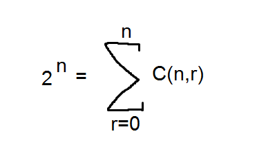
Also note that when constructing the next line, you will be using each number twice in the additions i.e. the left-most '1' on the 5th row gets used in making the left-most '1' on the 6th row (0+1) and also in making the left-most '5' on the 6th row (1+4). So you can expect that if you added all the combinations in each row, the number you get will be twice the number of the previous row. Considering we start at 1 when n=0, the added combinations will go 1, 2, 4, 8, 16, 32 etc. This means the sum of all combinations in the nth row will equal 2^n. In a formula this looks like:


Honestly, I don't know how much of a big deal that is, but I wanted to explore it because in one of my lectures the lecturer asked how many ways there were of making a subset of 5 elements (the first diagram in this post actually). I thought 'that's easy, just sum up all the combinations you can get when you have 0, 1, 2, 3, 4, or 5 slots (i.e. 32 combinations)' I was happy with myself when I got the answer right but when the lecturer explained the answer via the boolean table at the top of this post I thought 'oh that's a simpler way of looking at it, I wonder if there's a relationship between our two methods'. So how good is it that there indeed is a relationship here?

Alright so now hopefully you know what's up with combinations and permutations!

What's Up With Brute Force Algorithms?!

Ideally, when making an algorithm we want to find a way to grow the solution(s) ensuring the correct paths are taken to get to the right answer. This was seen in Dijkstra's algorithm where you want to find the shortest path from one vertex to another and the means of doing this is growing a path from the starting node and gradually learning more about the environment from visiting the other vertices. A brute force algorithm works almost in reverse: it starts off by generating all the possible solutions to the problem and then decides which ones are invalid (or which one is the best). In terms of Dijkstra's Algorithm, a brute alternative would be to generate all the possible paths from the start to the end (and we'll say no edge can be traversed twice to ensure we have a finite set of possible solutions at the end) and then scan through all the paths and calculate the total weight of them. Then the solution would be the path (or paths) with the lowest weight.

The problem with brute force algorithms is that they may require a lot of computation to generate all the possible permutations that create candidates for the solution. Looking at the graph from the blog on Dijkstra's Algorithm you can see that there are a holy-crap-that's-a-lot tonne of possible paths to take from vertex 0 to 4:

keep in mind this brute force algorithm, whilst generating the permutations, is blind to the conditions of the problem. If its job was to produce a sequence of vertices from 0 to 4, you're going to end up with 0-6 vertices inbetween. So you'll have:
0  4 //there's only one possibility with no vertices inbetween (P(6,0))
0  1  4 
0  2  4
0  3  4
0  5  4
0  6  4 
0  7  4 //there are 6 possibilities with 1 vertex inbetween (P(6,1))
0  1  2  4
0  1  3  4
0  1  5  4
0  1  6  4
0  1  7  4
0  2  1  4
0  2  3  4
0  2  5  4
0  2  6  4
0  2  7  4 
... // the amount with 2 vertices inbetween will end up being P(6,2) which is... let me see:

P(6,2) = 6!/(6-2)! = 6!/4! = 6 * 5 = 30 wow that's what I get for being lazy and thinking in terms of formulas when I could have just thought about the situation. The whole n!/(n-r)! is just another way of saying 'multiply n by (n-1) and then (n-2) and so on until you've got as many terms as there are positions for the vertices to take'. The (n-r)! just truncates the factorial to get what you want. If this isn't very clear don't worry I'll make a post on permutations and combinations soon. Anyway for now just think you've got 2 places and you've got 6 vertices to fill those places so for the first spot you have 6 to choose from and then you'll have 5 left to put in the second spot, equalling 6 * 5 = 30 permutations.

Anyway so we're going to end up with P(6,0)+P(6,1)+P(6,2)+P(6,3)+P(6,4)+P(6,5)+P(6,6) and what a good time it would be for some sigma notation:


Now 1957 doesn't seem like much (certainly not to a computer) but as you increase the number of vertices the number of permutations is going to explode (nothing grows like permutations). For example if you had 102 vertices in total which means 100 vertices that could show up between the start and end vertex, here's the number of permutations you'd get:

Have you ever had to decrease the font size in paint in order to fit a number in the frame? Because that's the level of permutational explosion we're talking about.

Now these permutations assume that the algorithm knows that the start and end vertex need to be at the start and end of the sequence in each permutation. If that restriction hadn't been imposed, the algorithm would be even more brutal (I'm using brutal here as an adjective to mean inconsiderate of the logic and restrictions of the system). There are different levels of brutality but the important fact is that the algorithm spits out all the possibilities within certain restrictions and then picks up the pieces, and the best way to improve on it is by incorporating known constraints into the permutation-generating part of the algorithm to cut down the possible solution set.

In terms of the brutal alternative to Dijkstra's Algorithm, 'picking up the pieces' refers to looking at which paths are actually possible and then deciding which path is the shortest. For determining whether a path is possible, the algorithm can go through the pairs of a given sequence much like a bubble sort, and determine whether there is an edge in the edge set, E, which contains the two vertices. If not, there's no link between them so it doesn't make sense to go directly from the first to the second vertex. So that particular sequence can get scrapped.

After a whole lot of computation, you'll be left with a set of possible solutions, where each possible solution is an actual path in the graph. Now all you have to do is go through each sequence again and compare each vertex and add the weight of their link to the total weight of that path. Then scan through the total weights and get the smallest one (like in the selection sort) and this is the solution. You could also mark the sequences which are equal to the minimum weight sequence so they can be added to the solution set (if there's multiple shortest paths) but you'll need to reset the list of minimum-length sequences as soon as you find a smaller sequence in the set. The process of finding the shortest path(s) can be done simultaneously with the process of finding which sequences aren't actually possible, but you're using a brute algorithm so clearly efficiency isn't your priority here.

So brute algorithms do a lot of number crunching when they 1) generate all the possible solutions and 2) whittle down these possible solutions to the actual solutions. These make them enormously inefficient but they get the job done (provided there are finite possible solutions), they're easy to make and for small amounts of possible states (here 1 sequence of vertices = 1 state) they aren't going to be overwhelmingly outperformed by more efficient algorithms.

I'll hopefully post a brute force solution to the famous Boat Problem soon because despite it being brute force, it's still very clever. Next up though (I've decided on it now) combinations and permutations!